# Shooter Location in meters from centre of wall
alpha <- 50
beta <- 70

# Number of shots
N <- 1000

# simulated firing angles
theta <- runif(n = N, min = -pi / 2, max = pi / 2)

# Hole locations in wall
x_k <- beta * tan(theta) + alphaBayesian numerical estimation of fat-tailed distributions
Can you find the hidden shooter?
analysis
R
bayesian
A palace in the middle of a fictional city is protected by a large wall. During the night, in protest, a citizen randomly opens fire at the palace walls with a machine gun from a fixed but hidden vantage point, riddling the long, straight palace walls with bullet holes. You are called in the morning to the Emperors office to analyse the bullet holes in the wall and determine where the shooter was firing from.

Main Takeaways
- There are many processes in the world that belong to heavy or fat tailed distributions.
- These are dangerous and difficult to work with.
- Often, simplifying assumptions (like gaussian approximation) can produce nice shortcuts, but when it goes wrong - it will go catastrophically wrong.
- Bayesian methods can give nice numerical approximations for solving these problems.
- Beware: They are very slow to converge.
Here is a rudimentary diagram
We can take any one bullet hole and reframe it mathematically:
From the diagram we express the unknown firing angle \(\theta\) for some shot, \(k\). The shooter is in position \((\alpha, \beta)\). We can express the following:
\[ tan (\theta_k) = \frac{x_k - \alpha}{\beta} \]
Giving the location along the wall \(x_k\) as:
\[ x_k = \beta tan(\theta_k) + \alpha \]
If we assume the bullets are sprayed uniformly (and angrily) across an angle of \(-\pi/2\) to \(\pi/2\) (-90° to 90°) we can simulate the bullet strike locations (\(x_k\)) for a known shooter location (\(\alpha\), \(\beta\)).
Let’s set the shooter location to 50m right of centre and 70m away from the wall. We will do this to generate the simulated bullet holes. When solving this, we won’t use these values directly, but rather we will try to recover them using a few analysis techniques.
data.frame(x = x_k) |>
    ggplot(aes(x)) +
    geom_histogram() +
    scale_x_continuous(limits = c(-500, 500)) +
    geom_vline(xintercept = alpha, lty = 2, col = "red") +
    theme_bw()
From above we assumed the shooting angle is uniformly distributed (rather than aimed at a specific narrow target). So the probability of a given firing angle is:
\[ p(\theta) = \frac{1}{\pi} \]
In order to find the probability density function for our bullet strikes \(p(x)\) we can use a rule to change the variable in a probability density function:
\[ p(x) = p(\theta)\lvert\frac{d\theta}{dx}\rvert \]
For the last part of this equation, we can take the derivative of both sides of \(\beta tan(\theta) = x - \alpha\) (see above) with respect to \(x\) giving:
\[ \beta sec^2(\theta) \times \frac{d\theta}{dx} = 1 \]
Doing some rearranging and using some trigonometric identities we get:
\[ p(x | \alpha, \beta) = \frac{1}{\pi \beta [1 + (\frac{x-\alpha}{\beta})^2]} \]
which happens to be the PDF of the Cauchy distribution.
The parameters for the Cauchy (location and scale parameters) correspond to our alpha and beta, which describe the horizontal and vertical coordinates of our shooter respectively.
We can visually overlay this on our simulated sample above to verify.
data.frame(x = x_k) |>
    ggplot() +
    geom_histogram(aes(x, y = ..density..)) +
    scale_x_continuous(limits = c(-500, 500)) +
    geom_function(fun = dcauchy, args = list(location = alpha, scale = beta), color = "blue", size = 1) +
    geom_vline(xintercept = alpha, lty = 2, col = "red") +
    theme_bw()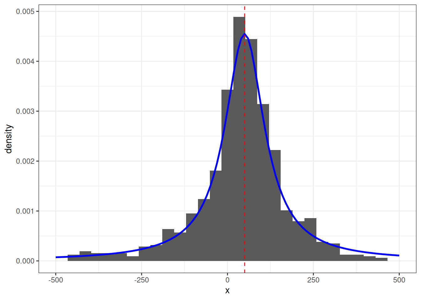
This is a problem as the Cauchy distribution, while stable, it has undefined mean and variance. The above histogram looks well behaved, but I have truncated the x-axis. It’s actually extremely heavy tailed. Below is the same data in all its glory.
data.frame(x = x_k) |>
    ggplot() +
    geom_histogram(aes(x, y = ..density..)) +
    # scale_x_continuous(limits = c(-500, 500)) +
    geom_vline(xintercept = alpha, lty = 2, col = "red") +
    theme_bw()
The implication here is that we cannot rely on the sample mean from a cauchy distribution to converge under the CLT to the true mean, so it’s unrelibale from an inference perspective. The existence of the fat-tails will prevent this convergence as seen below in the simulation. We can compare this, for reference, to the rapid convergence of samples from a standard normal distribution to its true mean.
There are a few sensible heuristics to overcome this such as relying on the mode/median estimates. Another way that is tricky but possible is to use maximum likelihood estimation.
I won’t do this directly, but you can easily plot the log-likelihood of the distribution over a grid of parameter values and get a good idea of what’s going on.
\[ \hat{\ell}(x_{1}, \dotsc, x_{n} \mid \alpha, \beta) = -n \log(\beta \pi) - \sum_{i=1}^{n} \log\left(1 + \left(\frac{x_{i} - \alpha}{\beta}\right)^{2}\right) \]
Interactive Charts
The below chart is interactive. Use your mouse to pan and zoom.
# Log-likelihood function
loglik <- function(x_k, alpha, beta) {
    -length(x_k) * log(beta * pi) - sum(log(1 + ((x_k - alpha) / beta)^2))
}

# Define grid of alpha and beta values
alphas <- seq(1, 100)
betas <- seq(1, 100)

# Compute over grid of parameters
grid <- outer(alphas, betas, Vectorize(function(alpha, beta) loglik(x_k, alpha, beta)))
normalised_grid <- matrix(exp(grid - max(grid)), nrow = length(alphas), ncol = length(betas))

# plot
persp3d(alphas,
    betas,
    normalised_grid,
    shade = 0.5, col = "light green",
    lit = TRUE, xlab = "Alpha", ylab = "Beta", zlab = "Log-Likelihood"
)
A fun way to try and solve this is using Bayesian inference. It would be hard (maybe not possible) to solve it analytically, but we can do this numerically using Hamiltonian Monte Carlo (or a close variant of this) via the stan language in R.
Below is the basic model. I can set an uninformative, uniform prior essentially over a 100m x 100m grid outside the palace gate.
data
{
    int<lower = 0> N;
    vector[N] x_k;
}
parameters
{
    real mu;
    real<lower = 0> sigma;
}
model
{
    // Priors
    mu ~ uniform(0, 100);
    sigma ~ uniform(0, 100);

    // Likelihood
    x_k ~ cauchy(mu, sigma);
}
# Simulated data
data_list <- list(N = N, x_k = x_k)
# Compile
model <- cmdstan_model(here::here("posts/2025-05-21-find-the-shooter/model.stan"))
fit <- model$sample(
data = data_list,
seed = 123,
chains = 4,
parallel_chains = 4,
iter_sampling = 1000,
iter_warmup = 500
)Running MCMC with 4 parallel chains...
Chain 1 Iteration: 1 / 1500 [ 0%] (Warmup)
Chain 1 Iteration: 100 / 1500 [ 6%] (Warmup)
Chain 1 Iteration: 200 / 1500 [ 13%] (Warmup)
Chain 1 Iteration: 300 / 1500 [ 20%] (Warmup)
Chain 1 Iteration: 400 / 1500 [ 26%] (Warmup)
Chain 1 Iteration: 500 / 1500 [ 33%] (Warmup)
Chain 1 Iteration: 501 / 1500 [ 33%] (Sampling)
Chain 1 Iteration: 600 / 1500 [ 40%] (Sampling)
Chain 1 Iteration: 700 / 1500 [ 46%] (Sampling)
Chain 1 Iteration: 800 / 1500 [ 53%] (Sampling)
Chain 1 Iteration: 900 / 1500 [ 60%] (Sampling)
Chain 1 Iteration: 1000 / 1500 [ 66%] (Sampling)
Chain 1 Iteration: 1100 / 1500 [ 73%] (Sampling)
Chain 1 Iteration: 1200 / 1500 [ 80%] (Sampling)
Chain 1 Iteration: 1300 / 1500 [ 86%] (Sampling)
Chain 1 Iteration: 1400 / 1500 [ 93%] (Sampling)
Chain 1 Iteration: 1500 / 1500 [100%] (Sampling) Chain 2 Iteration: 1 / 1500 [ 0%] (Warmup)
Chain 2 Iteration: 100 / 1500 [ 6%] (Warmup)
Chain 2 Iteration: 200 / 1500 [ 13%] (Warmup)
Chain 2 Iteration: 300 / 1500 [ 20%] (Warmup)
Chain 2 Iteration: 400 / 1500 [ 26%] (Warmup)
Chain 2 Iteration: 500 / 1500 [ 33%] (Warmup)
Chain 2 Iteration: 501 / 1500 [ 33%] (Sampling)
Chain 2 Iteration: 600 / 1500 [ 40%] (Sampling)
Chain 2 Iteration: 700 / 1500 [ 46%] (Sampling)
Chain 2 Iteration: 800 / 1500 [ 53%] (Sampling)
Chain 2 Iteration: 900 / 1500 [ 60%] (Sampling)
Chain 2 Iteration: 1000 / 1500 [ 66%] (Sampling)
Chain 2 Iteration: 1100 / 1500 [ 73%] (Sampling)
Chain 2 Iteration: 1200 / 1500 [ 80%] (Sampling)
Chain 2 Iteration: 1300 / 1500 [ 86%] (Sampling)
Chain 2 Iteration: 1400 / 1500 [ 93%] (Sampling)
Chain 2 Iteration: 1500 / 1500 [100%] (Sampling) Chain 3 Iteration: 1 / 1500 [ 0%] (Warmup)
Chain 3 Iteration: 100 / 1500 [ 6%] (Warmup)
Chain 3 Iteration: 200 / 1500 [ 13%] (Warmup)
Chain 3 Iteration: 300 / 1500 [ 20%] (Warmup)
Chain 3 Iteration: 400 / 1500 [ 26%] (Warmup)
Chain 3 Iteration: 500 / 1500 [ 33%] (Warmup)
Chain 3 Iteration: 501 / 1500 [ 33%] (Sampling)
Chain 3 Iteration: 600 / 1500 [ 40%] (Sampling)
Chain 3 Iteration: 700 / 1500 [ 46%] (Sampling)
Chain 3 Iteration: 800 / 1500 [ 53%] (Sampling)
Chain 3 Iteration: 900 / 1500 [ 60%] (Sampling)
Chain 3 Iteration: 1000 / 1500 [ 66%] (Sampling)
Chain 3 Iteration: 1100 / 1500 [ 73%] (Sampling)
Chain 3 Iteration: 1200 / 1500 [ 80%] (Sampling)
Chain 3 Iteration: 1300 / 1500 [ 86%] (Sampling)
Chain 3 Iteration: 1400 / 1500 [ 93%] (Sampling)
Chain 3 Iteration: 1500 / 1500 [100%] (Sampling) Chain 4 Iteration: 1 / 1500 [ 0%] (Warmup)
Chain 4 Iteration: 100 / 1500 [ 6%] (Warmup)
Chain 4 Iteration: 200 / 1500 [ 13%] (Warmup)
Chain 4 Iteration: 300 / 1500 [ 20%] (Warmup)
Chain 4 Iteration: 400 / 1500 [ 26%] (Warmup)
Chain 4 Iteration: 500 / 1500 [ 33%] (Warmup)
Chain 4 Iteration: 501 / 1500 [ 33%] (Sampling)
Chain 4 Iteration: 600 / 1500 [ 40%] (Sampling)
Chain 4 Iteration: 700 / 1500 [ 46%] (Sampling)
Chain 4 Iteration: 800 / 1500 [ 53%] (Sampling)
Chain 4 Iteration: 900 / 1500 [ 60%] (Sampling)
Chain 4 Iteration: 1000 / 1500 [ 66%] (Sampling)
Chain 4 Iteration: 1100 / 1500 [ 73%] (Sampling)
Chain 4 Iteration: 1200 / 1500 [ 80%] (Sampling)
Chain 4 Iteration: 1300 / 1500 [ 86%] (Sampling)
Chain 4 Iteration: 1400 / 1500 [ 93%] (Sampling)
Chain 4 Iteration: 1500 / 1500 [100%] (Sampling) Chain 1 finished in 0.1 seconds.
Chain 2 finished in 0.1 seconds.
Chain 3 finished in 0.1 seconds.
Chain 4 finished in 0.1 seconds.
All 4 chains finished successfully.
Mean chain execution time: 0.1 seconds.
Total execution time: 0.2 seconds.fit$summary() |>
knitr::kable(digits = 2)| variable | mean | median | sd | mad | q5 | q95 | rhat | ess_bulk | ess_tail |
|---|---|---|---|---|---|---|---|---|---|
| lp__ | -5615.07 | -5614.76 | 1.02 | 0.74 | -5617.11 | -5614.08 | 1 | 1821.00 | 2260.39 |
| mu | 49.22 | 49.27 | 3.14 | 3.16 | 44.06 | 54.38 | 1 | 3256.49 | 2405.38 |
| sigma | 69.43 | 69.34 | 3.19 | 3.21 | 64.37 | 75.00 | 1 | 3140.82 | 2484.86 |
We can see it has recovered the parameters mu and sigma. Which are used in stan to represent the location and scale parameters, which we have called \(\alpha\) and \(\beta\) representing the x and y axis locations of our shooter.
Below we can see an animation of the convergence of our sampling based on how many data points we used in the estimation.
Final thoughts
So a couple of things, firstly I have used 1000 data points to help generate my posterior samples. Is it reasonable that in this toy example the shooter would have unloaded 1000 rounds? No. It would still work with fewer data, but a key point here is how slow these estimates converge. I have picked a high number to easily demonstrate my point, but you can refer to the animation above to see how unstable it is with few data points. This is a reality in dealing with heavy-tailed distributions like the Cauchy. Looking at the same criticism from another perspective, the data generating process will produce outliers. How likely is it that our wall is thousands of meters long? Would we even detect the shots? Again, probably no. So you might ask why not just truncate the tails and approximate this process using a Gaussian? It would certainly give you easier to obtain estimates of the parameters and fewer headaches. The point here is it would work…until it didn’t. In fields like financial markets, using gaussian assumptions for fat tailed processes will likely make you look smart in the short term, but when it goes wrong it will go catastrophically wrong. Taleb discusses this at length in this book Statistical Consequences of Fat Tails.
Note: This is an adaptation of a well known problem called ‘Gull’s lighthouse problem’, first mentioned in the paper by Gull “Bayesian inductive inference and maximum entropy”1. There are loads of blog posts solving this, I haven’t done anything novel except enjoy replicating this by hand to learn a bit more. The mathematical derivation I have used comes from “Data Analysis: A Bayesian Tutorial” by Sivia and Skilling.2
Looking for a data science consultant? Feel free to get in touch here