★★★★★

Choosing an Airbnb using mathematical analysis of review data

Have you ever looked for a hotel, Airbnb, restaurant and checked out the reviews?

Always go for the highest rating right?

Sure..although that 5 star apartment only has 3 reviews…Ooo this one has more, oh but its only 4.72 stars…hmmm. Shit. What do I do?

We know higher reviews are better than lower reviews. But we also know more reviews are more reliable than fewer reviews.

Questions…

1. Can we somehow weight the review with how many reviews it has received?
   
2. Can we also include our own prior views on an item and have this influence our interpretation of the reviews?
   
3. Is there a way to quantify the likelihood of a bad experience despite a strong review?

Despite sounding wishy-washy, fortunately all of this can be resolved using common-or-garden variety techniques in a branch of statistics called Bayesian Analysis.

Example

Let’s say we are looking at a restaurant with 3 reviews of 4, 5, 5 on a 5-star scale.

Reviews are typically (but not always) just the arithmetic mean of all reviews received.

We have a average rating of 4.67 ★ (3).

We can add these up and view them as ‘total stars received’ out of ‘possible available stars’.

So we have 14 stars out of a possible 15. We can convert this to a proportion and call this our ‘success probability’ (14/15 = 0.9333).

We can now model this type of process using a mathematical distribution called a Binomial distribution.

\[ Y_i \sim Binomial(n_i, \theta_i) \] Where \(Y_i\) is the number of stars for something, \(n_i\) is the total number of stars possible and \(\theta_i\) is success probability.

The binomial process gives us a way to model or simulate how many stars would be most likely awarded out of 5 for an restaurant that usually scores (14/15 = 0.9333).

The reason we need a complicated mathematical way of doing this is because the expected result changes based on how much data we collect (just like how coin flips aren’t always 50/50 until we do a large number of flips).

Note

Actually, the support for a Binomial distribution is (0..n) but star ratings are usually only from 1 - 5 (with no zero-star reviews) so we need to shift our ‘star count’ to be the number of ‘stars above the minimum amount (1)’. So instead of our ratings accumulating 14 out of 15 stars, we actually model it as 11 ‘excess’ stars out of a possible 12. Another way of thinking about it is if we have 3 x one-star reviews. This is the lowest possible result but would look like we have a score of 3 out of 15 (3/15 = 0.2). So we need a way of making this be zero.

\[ Y'_i = \Sigma_{reviews} stars - n_i \\ \]

\[ Y'_i \sim Binomial(4n_i, \theta_i) \] Where \(n_i\) is the number of reviews.

So far we are assuming our success rate is fixed at 11 out of 12 (11/12 = 0.9166). But what if the next rating for this restaurant was a one-star. Now we have 4, 5, 5, 1. This gives us 11/16 excess stars = 0.6875. This is quite a drop. Obviously we only have a few ratings so our overall success will swing around wildly as new reviews come in.

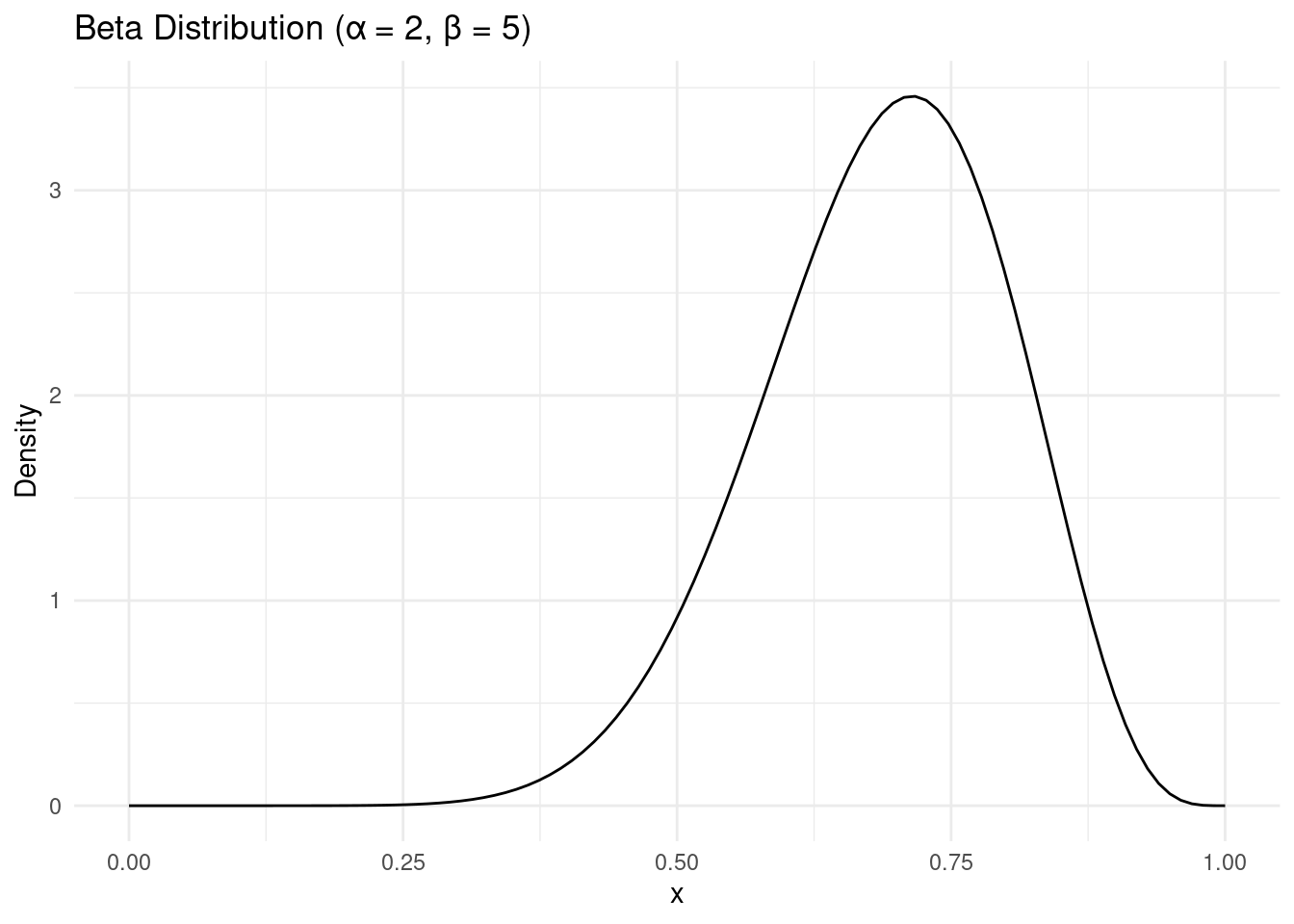
The key underpinning of Bayesian analysis is to not just plug in a single metric here, but to thoughtfully use a range of plausible options. Without further explanation (it’s boring), we are going to use another mathematical distribution called a Beta distribution to simulate a range of possible ‘success probabilities’. This distribution is bounded between zero and one and using the two hyper parameters we can adjust it’s shape to look like a plausible range of success probabilities.

\[ \theta_i \sim Beta(\alpha, \beta) \]

An example probability distribution that approximates a range of values around 0.7 with a slight negative skew

If we simulate lots of draws from this distribution we can then feed them into our binomial model and simulate ratings data under a range of input conditions. Why is this good?

1. As we accumulate more ratings information, the spread of this curve gets narrower and we gain more confidence in what we think the ‘true’ star success proportion is.
   
2. We can start the process by making up a Beta distribution that reflects our best-guess in lieu of actual ratings. This might be totally uninformative if we have no clue how good a product is, or we might have strong view that it’s going to be highly rated based on word of mouth or previous products.

The above point (2) is why we might insist on buying a new product and ignore its poor initial ratings if we think it might be good anyway.

Choosing an Airbnb

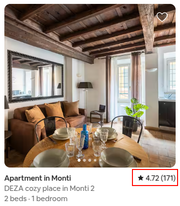
So back to the Airbnb example from the picture above.

Firstly, the Monticiano apartment is just rated better than the DEZA apartment. No amount of mathematical trickery can reverse that. There are a few things we can do to try and calculate how much overlap there is in the possible ratings outcomes. But I’m going to ask a different question:

I don’t care if it’s 5 star or 4.72 stars. I just really don’t want a bad experience (say, 3 rating or less). Given the current ratings (and the inherent uncertainly in the ratings), what is the probability I will have a 3 star or worse stay?

I have written some basic code to calculate that for me below.

# What is the simulated probability that I will have a 3 star night (or worse). 

bad_experience_prob <- function(a = 1, b = 1, rating, n_reviews, rating_threshold, n_sim = 10000){
  
  # adjusted star ratings
  n_stars_gt_min <- rating*n_reviews - n_reviews
  n_total <- n_reviews * 4
  
  # update prior
  alpha <- n_stars_gt_min + a
  beta <-  (n_total - n_stars_gt_min) + b

  # posterior predictions
  beta_samples <- rbeta(n = n_sim, shape1 = alpha, shape2 = beta) 
  posterior_samples <- rbinom(n = n_sim, size = 4, prob = beta_samples) + 1
  
  prob_bad <- mean(posterior_samples <= rating_threshold)
  
  return(prob_bad)
  
  }

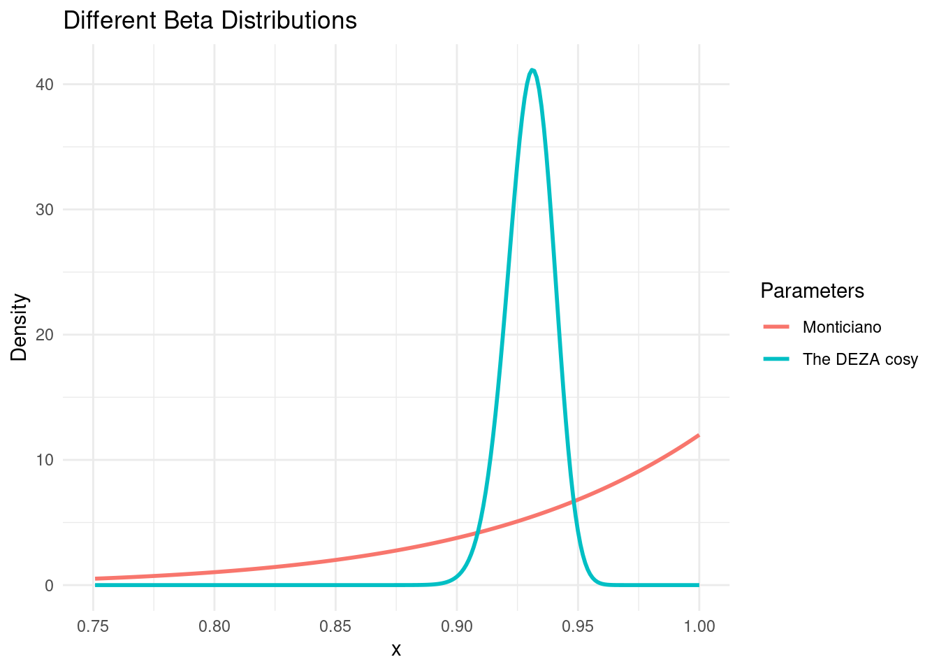
The Monticiano apartment with ★ 5.0 (3):

Results:  

Based on 10,000 simulated ratings.

With a ★ 5.0 (3) rating, assuming no prior view on the quality, the chance of a three star rating or worse is:  
4.53%

The DEZA cosy place in Monti with ★ 4.72 (171):

Results:  

Based on 10,000 simulated ratings.

With a ★ 4.72 (171) rating, assuming no prior view on the quality, the chance of a three star rating or worse is:  
2.57%

So despite having a higher rating, the first apartment has a 4% chance of a bad experience, double that of the other apartment.

Why? Well despite having a higher mean success rate, just the 3 ratings introduces lots of uncertainly which helpfully propagates to our simulations.

Comparing the posterior distribution of both apartments

This all begs the question (at least for me) if we can visualise this probability surface for all combinations of ratings and review strength.

Below we can see that as the average ratings get below 3, its obviously expected to increase the odds of a bad (< 3 star) experience. There is an interesting lip when we look at the curve where review numbers are very small. Let’s zoom in.

Interactive Charts

The below charts are interactive. Use your mouse to pan and zoom.

Anything can happen we we only have one or two reviews, but things stabilise very quickly as we approach 10, 20 and 30 reviews.

When we focus on just 4.5 - 5 star rated products, we can locate situations where say a 4.8 star review with 5 reviews would yield the same risk of a bad experience as a 4.6 with 20 reviews etc.

Key Takeaway

Good decision making probably requires more than just acting on a single metric alone, and some context around the uncertainty of that metric can help with making stronger, empirical decisions.

If you are working with review data, you need to have the tools to model and analyse more than just biggest number wins.

Further thoughts

There are a few different directions you could keep taking this. There are certainly different modelling approaches.I didn’t explain much about the selection of a prior distribution, which is very important in Bayesian analysis. Arguably the prior for consumer ratings wouldn’t share the nice normal convergence properties of a Beta distribution. It’s probably more bimodal with a tendency to see spikes at 1 star and 5 star. This would require mores sophisticated computational methods that I can’t be bothered with right now.

For more info on the maths behind this type of work you can check out this good accessible and free resource: Probability and Bayesian Modeling

Looking for a data science consultant? Feel free to get in touch here